Justdail SCAM calls | Justdail product enquiry scam | Fraud Alert on Justdail | Indiamart SCAM calls

DO NOT PAY IN ADVANCE

Aaiya aaj baat krte h new scam/fraud ki jo ki JustDail/Indiamart jaisi websites ko use krke ho rha h. Jaise hi hum log koi product enquiry ke liye apna number submit krte h humme Justdail se call anne start ho jate h. Vo log apko apne rates btayege or whatsapp pe apni or company ki details bhejege jo ki sb fake hongi. Fake GST and fake address. Please google and justdail pe review check krle ekbaar jarur. Ye log apko kaffi low proce offer krege or payment advance bolege. 

M kuch image daalrha hun inki fake details ki or sathme kuch numbers jo ye log use kr rhe h:

Gujrat Paper Products.

Shree Shyam Paper Mart. 

Manufactarercompany8 

K COPIAR PAPER FROM MUDRAMOOLA PAYYAAMPALLY PU PALLY ROAD PAYYAAMPALLY WAYANAD KERALA PIN CODE 670645 MOBILE NUMBER +919001872982 GST NUMBER 32BXIPV8253L1ZT 

Phone Numbers: 

7878319002 

9001872982 

9694931769 

8114420394 

8068658663 

6350516416 

9694931769 

 Images:

How to vlookup values across multiple worksheets? | VLOOKUP Formula in Excel with Multiple Sheets | Match value across multiple sheets in excel

We can achieve this using INDIRECT function is excel.

Vlookup multiple sheets with INDIRECT:

To use this array formula, you should give these three worksheets a range name, please list your worksheet names in a new worksheet, such as following screenshot shown:

1. Give these worksheets a range name, select the sheet names, and type a name in the Name Box which next to the formula bar, in this case, I will type Sheetlist as the range name, and then press Enter key.

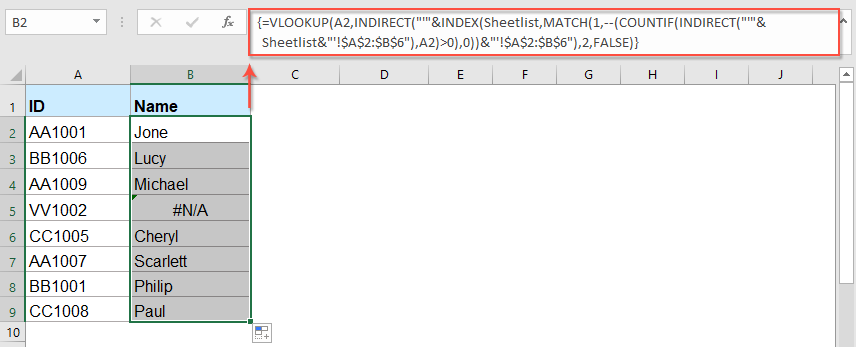
2. And then you can enter the following long formula into your specific cell:

=VLOOKUP(A2,INDIRECT("'"&INDEX(Sheetlist,MATCH(1,--(COUNTIF(INDIRECT("'"&Sheetlist&"'!$A$2:$B$6"),A2)>0),0))&"'!$A$2:$B$6"),2,FALSE)

Example 2:

=VLOOKUP($V2,INDIRECT("'"&INDEX(Lookup_sheets,MATCH(1,--(COUNTIF(INDIRECT("'"&Lookup_sheets&"'!$A$2:$B$300"), $V2)>0), 0))&"'!$A$2:$B$300"), 2, FALSE)

3. And then, press Ctrl + Shift + Enter keys together to get the first corresponding value, then drag the fill handle down to the cells that you want to apply this formula, all the relative values of each row have been returned as follows:

Notes:

1. In the above formula:

• A2: is the cell reference which you want to return its relative value.
• Sheetlist/Lookup_sheets: is the range name of the worksheet names.
• A2:B6: is the data range of the worksheets you need to search.
• 2: indicates the column number that your matched value is returned.

2. If the specific value you lookup doesn't exist, a #N/A value will be displayed. if you want to replace #N/A with specific value this can be handled with IFNA as shown below:

=IFNA(VLOOKUP($V2,INDIRECT("'"&INDEX(Lookup_sheets,MATCH(1,--(COUNTIF(INDIRECT("'"&Lookup_sheets&"'!$A$2:$B$300"), $V2)>0), 0))&"'!$A$2:$B$300"), 2, FALSE),"Not Found")