We can achieve this using INDIRECT function is excel.
Vlookup multiple sheets with INDIRECT:
To use this array formula, you should give these three worksheets a range name, please list your worksheet names in a new worksheet, such as following screenshot shown:

1. Give these worksheets a range name, select the sheet names, and type a name in the Name Box which next to the formula bar, in this case, I will type Sheetlist as the range name, and then press Enter key.

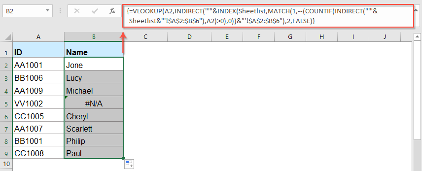
2. And then you can enter the following long formula into your specific cell:
3. And then, press Ctrl + Shift + Enter keys together to get the first corresponding value, then drag the fill handle down to the cells that you want to apply this formula, all the relative values of each row have been returned as follows:

Notes:
1. In the above formula:
- A2: is the cell reference which you want to return its relative value.
- Sheetlist/Lookup_sheets: is the range name of the worksheet names.
- A2:B6: is the data range of the worksheets you need to search.
- 2: indicates the column number that your matched value is returned.
2. If the specific value you lookup doesn't exist, a #N/A value will be displayed. if you want to replace #N/A with specific value this can be handled with IFNA as shown below:
=IFNA(VLOOKUP($V2,INDIRECT("'"&INDEX(Lookup_sheets,MATCH(1,--(COUNTIF(INDIRECT("'"&Lookup_sheets&"'!$A$2:$B$300"), $V2)>0), 0))&"'!$A$2:$B$300"), 2, FALSE),"Not Found")